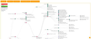
통계적 검정은 품질 및 제조 분야에서 의사결정에 객관적인 근거를 제공하는 유일한 방법입니다. 이를 통해 공정상의 변동을 파악하고 무작위적인 변동과 실제 문제를 구분할 수 있습니다. 엔지니어링 분야에서는 통계를 활용하여 시스템 성능의 패턴, 이상치, 그리고 고장 원인을 식별함으로써 데이터 기반 의사결정을 지원합니다. 실험 결과를 엄격하게 분석함으로써 엔지니어는 제품 설계 및 제조 공정을 검증하고 구현 전에 잠재적인 문제를 발견할 수 있습니다. 이러한 체계적인 접근 방식은 예상치 못한 고장의 위험을 줄이고 신뢰성을 보장하며 국제 안전 기준을 준수함으로써 전반적인 안전성을 향상시킵니다.
이 글에서는 제조 분야에서 사용되는 주요 통계 검정들을 검토하고… 전사적 품질 관리 (TQM).
참고: 다음 두 가지 통계 테스트 및 분석은 공학, 연구 및 과학과도 관련이 있으므로 함께 제시합니다.
- 상관 분석: 두 변수 간의 관계의 강도와 방향을 측정합니다(예: 피어슨 상관계수).
- 회귀 분석: 단순 선형 회귀 분석부터 다중 회귀 분석까지, 변수(예: 입력 요소와 공정 출력) 간의 관계를 조사합니다.
이 내용은 여기에 포함되어 있지 않지만, 엔지니어링 분야의 주요 알고리즘 10가지에 대한 특정 기사에 자세히 설명되어 있습니다.
정규성 검정

통계 검정 분야에서 흔히 사용되는 많은 통계 방법(t-검정, 분산 분석, 선형 회귀 분석 등)은 데이터가 정규 분포를 따른다고 가정합니다(또는 잔차/오차가 정규 분포를 따른다고 가정합니다). 이러한 가정을 위반하면 결과가 신뢰할 수 없게 될 수 있습니다. p값이 오해의 소지가 생기고, 신뢰 구간이 잘못될 수 있으며, 제1종/제2종 오류의 위험이 증가합니다. 다만, 일원 분산 분석과 같은 일부 검정은 비정규 분포도 비교적 잘 처리할 수 있습니다.
참고: 데이터가 정규 분포를 따르지 않는 경우(아래 실제 사례 참조), 정규 분포를 가정하지 않는 비모수 검정(예: Mann-Whitney U 검정 또는 Kruskal-Wallis 검정)을 사용하거나 데이터를 변환해야 할 수 있습니다. 하지만 이러한 방법은 이 글의 범위를 벗어납니다.
이를 위한 여러 통계적 검정 방법이 있지만, 여기서는 특히 표본 크기가 작은 경우(일반적으로 n < 50)에 유용하지만 최대 2000까지 사용할 수 있는 샤피로-윌크 검정에 대해 자세히 설명하겠습니다.
참고로, 다른 일반적인 정규성 검사는 다음과 같습니다.
- 콜모고로프-스미르노프(KS) 검정(릴리포스 보정 적용): 표본 크기가 클수록 성능이 우수하며, 특히 소규모 데이터셋의 경우 샤피로-윌크 검정보다 민감도가 낮습니다.
- 앤더슨-달링 검정: 모든 표본 크기에 적합하며, 분포의 꼬리 부분(극단값)에서 민감도가 높고, 극단값에서 정규성에서 벗어나는 것을 감지하는 데 더 강력한 검정력을 갖습니다.
샤피로-윌크 정규성 검정 수행 방법
1. 샤피로-윌크 검정 통계량(W)을 계산하십시오. [latex]W = \frac{\left(\sum_{i=1}^{n} a_i x_{(i)}\right)^2}{\sum_{i=1}^{n} (x_i – \bar{x})^2}[/latex] Note: as the calculation of the [latex]a_i[/latex] coefficients is nontrivial and generally requires a table or algorithm, which is why the Shapiro-Wilk test is nearly always computed by software such as R, Python’s SciPy, MS Excel add-ons or other dedicated softwares. 수동 계산을 원하시면 이 페이지를 참조하세요. provides all the [latex]a_i[/latex] coefficients and p-value for samples up to 50. W 값은 0에서 1 사이의 값을 가지며, W = 1은 완벽한 정규성을 나타내고, W < 1은 1에서 멀어질수록 데이터의 정규성이 떨어진다는 것을 의미합니다. 2. W 값만으로는 충분하지 않습니다. 신뢰 수준을 얻으려면 해당 p값과 함께 사용해야 합니다. 샤피로-윌크 표에서, n개의 샘플 크기를 갖는 행에서 계산된 W 값에 가장 가까운 값을 찾아 해당 값을 가져옵니다. 상단에 있는 p값 | 분자는 가중치가 부여된 정렬된 표본 값의 제곱합을 나타냅니다. 분모는 표본 평균으로부터의 제곱 편차의 합(즉, 표본 분산을 (n-1)로 나눈 값)입니다. [latex]x_{(i)}[/latex] = the i-th order statistic (i.e., the i-th smallest value in the sample) [latex]x_i[/latex] = the i-th observed value [latex]\bar{x}[/latex] = the sample mean [latex]a_i[/latex] = constants (weights) calculated from the mean, variances, and covariances of the order statistics of a sample from a standard normal distribution ((N(0,1))), and depend only on n (sample size). n = 표본 크기 |
3. 결과: p값이 선택된 유의수준(예: 0.05)보다 크면, 검정 대상 데이터가 정규분포를 따른다는 통계적 근거가 있다고 볼 수 있습니다. | |
정규성 검정을 위해서는 수치적 방법과 헨리 선, QQ 플롯 또는 히스토그램과 같은 그래프적 방법을 함께 사용하는 것이 흔히 권장됩니다.
비정규 분포에 주의하세요!
정규/가우스 분포가 가장 흔한 경우이지만, 자동으로 가정해서는 안 됩니다. 일상적으로 접하는 반례는 다음과 같습니다.
- 개인 간의 부와 소득 분배는 파레토 분포(멱법칙 분포)를 따르며, 매우 부유한 사람들이 긴 꼬리 형태로 분포하는 비대칭적인 형태를 보인다.
- 한 국가의 도시 인구 규모는 소수의 매우 큰 도시와 다수의 작은 마을로 구성된 지프의 법칙(멱법칙)을 따른다.
- 지진의 규모와 빈도는 멱법칙/구텐베르크-리히터 분포를 따릅니다. 즉, 작은 지진은 흔하고 큰 지진은 드뭅니다.
- 금융 시장의 일일 가격 변동 또는 수익률은 가우시안 분포가 아닌 두꺼운 꼬리 분포를 따르며, 정규 분포에서 예측하는 것보다 큰 편차가 더 자주 발생합니다.
- 언어에서 단어의 빈도는 위의 도시 인구 분포와 마찬가지로 지프의 법칙(멱법칙)을 따릅니다. 즉, 자주 사용되는 단어는 소수이고, 대부분의 단어는 드물게 사용됩니다.
- 인터넷 트래픽/웹사이트 인기: 멱법칙/롱테일: 일부 사이트는 수백만 건의 조회수를 기록하지만, 대부분의 사이트는 조회수가 매우 적습니다.
- 컴퓨터 시스템의 파일 크기는 로그 정규 분포 또는 멱법칙 분포를 따르며, 매우 큰 파일 몇 개와 작은 파일 다수로 구성됩니다.
- 인간 수명/장수: 오른쪽으로 치우친 분포 (모델링 가능) 와이블 (곰페르츠 분포와 같은) 정규 분포가 아니며, 고령층에서 사망률이 더 높습니다.
- 소셜 네트워크 연결은 멱법칙을 따른다. 소수의 사용자는 많은 연결을 갖고 있고, 대부분의 사용자는 적은 연결을 갖고 있다.
이러한 분포의 대부분은 '큰 값은 적고 작은 값은 많다'는 특징을 가지며, 멱법칙, 두꺼운 꼬리, 지수 분포 또는 로그정규 분포와 같은 특징을 보이고, 가우시안 분포처럼 대칭적인 형태를 띠지는 않습니다.
t-검정(스튜던트 t-검정)
1908년 윌리엄 실리 고셋이 '스튜던트'라는 가명으로 개발한 t-검정(또는 '스튜던트의 t-검정')은 표본 크기가 작고 모집단 분산을 알 수 없을 때 평균을 비교하는 데 사용되는 통계 검정입니다. 두 모집단의 평균을 비교하는 데 초점을 맞추고 있으며, 제조업 분야에서 가장 널리 사용되는 검정 중 하나입니다.

목적: t-검정은 엔지니어와 품질 전문가가 두 그룹의 평균 간 또는 표본 평균과 알려진 표준 간에 통계적으로 유의미한 차이가 있는지 판단하는 데 도움이 됩니다. 이는 일반적으로 공정 변경이나 제품 수정이 효과가 있는지 평가하기 위한 가설 검정에 사용됩니다. ~ 주도의 우연에 의해 예상되는 것 이상의 실질적인 개선이나 차이를 가져옵니다.
업계의 실제 사례:
- 자동차 제조에서 t-검정은 서로 다른 두 공급업체의 강철 인장 강도를 비교하여 일관된 품질을 보장하는 데 사용될 수 있습니다.
- 제약 분야에서 t-검정은 새로운 생산 공정이 표준과 유의미하게 다른 평균 중량의 정제를 생산하는지 분석하는 데 사용됩니다.
- 전자공학에서 엔지니어는 t-검정을 사용하여 특정 조건이 충족되는지 확인할 수 있습니다. 디자인 변경 에서 회로 기판 그 결과 전기 저항이 눈에 띄게 향상됩니다.
학생 t-검정 방법
t-검정에는 여러 변형이 있지만, 여기서는 두 개의 서로 다른 생산 배치에서 추출한 샘플을 비교하는 소위 '비대응' 버전의 '두 표본 t-검정'에 초점을 맞추겠습니다.
- 귀무가설과 대립가설을 명시하십시오. 이 예시에서는 '평균 간에 차이가 없다'와 '평균 간에 차이가 있다'입니다.
- 비교 대상인 두 생산 배치에서 데이터를 수집하고 계산하세요.
- the 2 sample means [latex]\bar{X} = \frac{1}{n_1} \sum_{i=1}^{n_1} X_i[/latex] and [latex]\bar{Y} = \frac{1}{n_2} \sum_{j=1}^{n_2} Y_j[/latex]
- Calculate the 2 sample variances: [latex]S_X^2 = \frac{1}{n_1-1} \sum_{i=1}^{n_1} (X_i – \bar{X})^2[/latex] and [latex]S_Y^2 = \frac{1}{n_2-1} \sum_{j=1}^{n_2} (Y_j – \bar{Y})^2[/latex]
- 표본 크기.
- 검정 통계량을 계산합니다. 이 방법은 두 표본이 서로 독립적이고 두 표본 모두 정규 분포를 따르는 모집단에서 추출되었다고 가정하지만, 여전히 두 가지 경우가 있습니다.
- 등분산 가정 시 (“pooled” t-test;): Pooled variance: [latex]S_p^2 = \frac{ (n_1-1)S_X^2 + (n_2-1)S_Y^2 }{ n_1 + n_2 – 2 }[/latex]
Test statistic: [latex]t = \frac{ \bar{X} – \bar{Y} }{ S_p \sqrt{ \frac{1}{n_1} + \frac{1}{n_2} } }[/latex] - 분산이 같지 않은 경우 (Welch’s t-test): Test statistic: [latex]t = \frac{ \bar{X} – \bar{Y} }{ \sqrt{ \frac{S_X^2}{n_1} + \frac{S_Y^2}{n_2} } }[/latex] Degrees of freedom (approximate, Welch-Satterthwaite): [latex]df = \frac{\left( \frac{S_X^2}{n_1} + \frac{S_Y^2}{n_2} \right)^2}{ \frac{ (S_X^2 / n_1)^2 }{ n_1 – 1 } + \frac{ (S_Y^2 / n_2)^2 }{ n_2 – 1 } }[/latex]
- 등분산 가정 시 (“pooled” t-test;): Pooled variance: [latex]S_p^2 = \frac{ (n_1-1)S_X^2 + (n_2-1)S_Y^2 }{ n_1 + n_2 – 2 }[/latex]
- Use the calculated ( t ) and degrees of freedom ([latex]n_1+n_2-2[/latex] for equal variances, or the Welch formula) to look up or compute the p-value from the t-distribution (depending on whether it’s a one-tailed or two-tailed test).
- 결과: 계산된 t값을 선택한 신뢰 수준과 자유도에 따른 통계표의 임계 t값과 비교하거나, p값을 계산하는 소프트웨어를 사용하십시오. t 통계량이 임계값을 초과하거나 p값이 임계값(일반적으로 0.05)보다 낮으면 귀무 가설을 기각합니다.
링크 t-검정 임계값 표
The F-Test
The F-test, introduced by statistician Ronald A. Fisher in the early 20th century, is used to compare the variability (variance) between two sets of data, to assess if their population variances are significantly different. In quality and engineering, it often helps determine if process changes or different machines produce consistent results or if new methods affect product variability. Often a preliminary step before applying t-tests and ANOVA on larger comparisons.
목적: the F-Test is used to confirm if two processes or samples have the same level of variation, which supports quality control decisions and process improvements. It helps engineers identify if changes (e.g., new machines, suppliers, or materials) impact the consistency or quality of a product.
Industry Examples
- Manufacturing: comparing the dimensional variances of parts produced by two different machines to ensure both machines produce consistently within quality standards.
- Supplier Evaluation: comparing the strength variability of raw materials from two different suppliers to decide if one supplier provides more consistent quality.
- Quality Improvement: testing if a process improvement (like a new calibration method) has reduced the variability in final product weight compared to the old method.
How-to the F-Test
- Collect two sets of sample data (e.g., measurements from process A and process B).
- Calculate the variance for each sample group A and B.
- Divide the larger variance by the smaller variance to get the F-value.
- 결과: compare this F-value to a critical value from the F-distribution table based on sample sizes and the desired confidence level; if the calculated F-value is greater, the variances are significantly different. In statistical tests, the variance ratio tests, the degrees of freedom (DOF) associated with each group is the quantity of samples minus one (note that this is different for an ANOVA result comparison).
F-distribution table: link to the F-distribution table up to 15×15 DOF (and online F critical calculator for bigger DOF)
분산 분석(ANOVA)
While the F-test above refers broadly to any statistical test that uses the F-distribution and is used to compare variances or ratios of variances between two or more groups, the ANOVA is a variant that compares the means of three or more groups to see if at least one is significantly different. The ANOVA test was also developed by Ronald Fisher in the 1920s as a statistical tool for agricultural experiments.
목적: the Analysis of Variance (ANOVA) is to determine whether there are statistically significant differences between the means of three or more independent groups. In quality, engineering and particularly in 실험 설계(DOE), it helps identify which factors or processes have a significant impact on product performance or output, aiding robust decision-making and process improvement.
예시:
- In pharmaceutical production, ANOVA can help compare the effects of different formulation processes on the efficacy of a drug.
- In electronics, it is used to test if the variance in circuit board failure rates is due to different batches of raw materials.
How-to ANOVA in Brief
1. Define the groups or treatments you want to compare and collect data from each group. Calculate
2. Use these values to calculate the F-statistic (see on the right), which is the ratio of variance between groups to the variance within groups. 3. Compare F-statistic to a critical value from the F-distribution table at a chosen significance level (like 0.05). 4. Result: if the F-statistic exceeds the critical value, you conclude that there are significant differences among group means. | The F-statistic: The F corresponds to the Mean Square Between Groups (MSB) divided by Mean Square Within Groups (MSW) Practically: [latex]F = \frac{ \frac{SSB}{k-1} }{ \frac{SSW}{N-k} }[/latex] SSB = Sum of Squares Between Groups |
The Chi-Square Test
The Chi-Square Test, introduced by Karl Pearson in 1900, revolutionized statistical hypothesis testing by providing a method to determine if there is a significant difference between expected and observed frequencies in categorical data. In quality and engineering, it helps assess whether deviations in a process or product attributes occur by chance or suggest a systemic issue.
목적: the Chi-Square Test checks if the differences between observed and expected results in quality measurements are due to random variation or indicate a specific problem that needs addressing.
Practical examples in industry
- Manufacturing Defects: checking if the distribution of defective products across different shifts or machines is uniform, and whether certain shifts have a significantly higher defect rate.
- Supplier Quality: comparing the quality performance (e.g., pass/fail rates) of components from multiple suppliers to determine if one supplier’s parts are statistically more likely to fail.
- Customer Complaints: analyzing whether the types or frequency of customer complaints are randomly distributed throughout the year, or are associated with specific times, products, or regions.
How to do the chi-square test
- Collect observed data and determine the expected frequencies for each category under the null hypothesis.
- Use the Chi-Square formula: Χ² = Σ[(O – E)² / E] where O is observed, E is expected.
- Compare the calculated Chi-Square value against a critical value from the Chi-Square table with the appropriate degrees of freedom.
- 결과: if the value exceeds the table value, conclude there is a statistically significant difference.
Link to the chi-square critical values table
Chi-Square Full Example: Fairness of a Dice
| 나 | Oi | Ei | Oi−Ei | (Oi−Ei)2 |
| 1 | 5 | 10 | −5 | 25 |
| 2 | 8 | 10 | −2 | 4 |
| 3 | 9 | 10 | −1 | 1 |
| 4 | 8 | 10 | −2 | 4 |
| 5 | 10 | 10 | 0 | 0 |
| 6 | 20 | 10 | 10 | 100 |
| Sum | 134 | |||
This full example is taken from Wikipedia Chi-square article.
Experience: a 6-sided die is thrown 60 times. The number of times it lands face up on 1, 2, 3, 4, 5, 6 is 5, 8, 9, 8, 10 and 20, respectively.
Question: is the die biased, according to the Pearson’s chi-squared test at a significance level of 95% and/or 99%?
The null hypothesis is that the die is unbiased, hence each number is expected to occur the same number of times, in this case, 60/n = 10.
The outcomes can be tabulated as on the right:
| Degrees of freedom | Probability less than the critical value | ||||
|---|---|---|---|---|---|
| 0.90 | 0.95 | 0.975 | 0.99 | 0.999 | |
| 5 | 9.236 | 11.070 | 12.833 | 15.086 | 20.515 |
Looking at an upper-tail critical values of chi-square distribution table (table linked in the how-to above), the tabular value refers to the sum of the squared variables each divided by the expected outcomes.
For the present example, this means χ2=25/10+4/10+1/10+4/10+0/10+100/10=13.4
Conclusion of test: this 13.4 is the experimental result whose unlikeliness (with a fair die) we wish to estimate, with a significance or confidence between 97.5% and 99%
Process Capability (Cp, Cpk, Pp, Ppk)

Not a statistical test per se, these 4 ratios assess how well a process meets specifications, thus becoming a critical tool for maintaining and improving quality standards in manufacturing.
Process capability analysis originated in the early 20th century alongside the rise of statistical quality control in manufacturing, pioneered by figures like Walter Shewhart. Its methods evolved through the growth of 식스 시그마 and Total Quality Management (TQM) in the late 20th century as a cornerstone of modern quality engineering.
목적: process capability analysis assesses how well a process can produce output within specified limits (tolerances). It quantifies the variability of a process relative to design specifications and determines the likelihood of producing defective products. The analysis helps identify opportunities for process improvement and ensures products consistently meet customer requirements.
Cp, Cpk and Statistical Tests in Industry
- Automotive manufacturing: statistical tests and these 4 ratios are used to check whether the diameter of engine pistons remains consistently within tight tolerance limits, ensuring compatibility and reducing engine failures.
- Pharmaceutical industry: applied to verify that the fill weight of tablets or capsules consistently meets regulatory and quality standards, minimizing underdose or overdose risks.
- 반도체 manufacturing: employed to monitor the thickness of wafer coatings, ensuring reliability and performance in microchip production.
How to calculate Cp, Cpk, Pp and Ppk
Cp: Process Capability
| [latex]Cp = \frac{USL – LSL}{6\sigma}[/latex] | USL = Upper Specification Limit LSL = Lower Specification Limit σ = standard deviation (typically estimated from within-subgroup variation) |
Cpk: Process Capability Index
[latex]Cpk = \min\left(\frac{USL – \mu}{3\sigma}, \frac{\mu – LSL}{3\sigma}\right)[/latex] | [latex]\mu[/latex] = process mean |
Pp: Process Performance
[latex]Pp = \frac{USL – LSL}{6s}[/latex] | [latex]s[/latex] = overall standard deviation (includes both within and between subgroup variations; used over a longer period) |
Ppk: Process Performance Index
[latex]Ppk = \min\left(\frac{USL – \bar{x}}{3s}, \frac{\bar{x} – LSL}{3s}\right)[/latex] | [latex]\bar{x}[/latex] = overall mean |
How to Conclude with Cp, Cpk, Pp, Ppk Values
- Cp, Pp: if >1, the process has the potential to meet specifications; values ≥1.33 are generally considered capable, depending o your industry and the criticality of your exact application
- Cpk, Ppk: these reflect how centered the process is within specs; the closer Cpk/Ppk are to Cp/Pp, the more centered the process.
- If Cpk or Ppk <1, a significant portion of output is likely outside the specification; process improvement is needed.
- A higher index indicates a more capable (and usually, higher quality) process.
Conclusion & Pitfalls
Statistical tests are powerful tools in data analysis, but their use demands both strong theoretical understanding and critical real-world judgment and adaptation, far from just a statistical software installation or QMS rules.
- Understanding assumptions & selecting the right test: every statistical test has a set of underlying assumptions (e.g., normality of data, equal variances, independence of observations). If these assumptions are violated or an inappropriate test chosen, the results of the test may be invalid or misleading.
- Real-world messiness & business context matters: industrial data often violate test assumptions (e.g., non-normality, autocorrelation). Blindly applying textbook tests can result in completely misleading analyses.
- Data quality issues: measurement errors, outliers, and missing data are common in industrial statistical tests and must be addressed and documented before testing.
For product design so as for quality, put your effort where needed: “Sometimes, results are statistically significant but have negligible practical impact, or vice versa”
External Links on Statistical Tests for Quality
국제 표준
(링크 위에 마우스를 올려놓으면 콘텐츠에 대한 설명을 볼 수 있습니다.)
사용된 용어집
Analysis of Variance (ANOVA): 세 개 이상의 독립적인 집단의 평균 간에 유의미한 차이가 있는지 판단하기 위해 집단 내 및 집단 간 분산을 분석하는 통계적 방법입니다. 이는 하나 이상의 요인이 종속 변수에 미치는 영향을 평가합니다.
Degrees Of Freedom (DOF): 기계 시스템 또는 통계 모델의 구성을 정의하는 독립적인 매개변수의 수를 나타내는 척도로, 시스템이 제약 조건을 위반하지 않고 움직이거나 변할 수 있는 방법의 수를 의미합니다.
Design of Experiments (DOE): 여러 변수가 반응 변수에 미치는 영향을 평가하기 위해 통제된 시험을 계획, 수행, 분석 및 해석하는 체계적인 방법으로, 공정이나 제품을 최적화하고 이해할 수 있도록 해준다.
Design of Experiment (DOE): a systematic method for planning, conducting, and analyzing controlled tests to evaluate the effects of multiple variables on a response variable, facilitating the identification of optimal conditions and interactions among factors.
Process Capability Index (Cpk): a statistical measure that quantifies how well a process can produce output within specified limits, indicating the relationship between the process mean and the nearest specification limit, adjusted for process variability.
Process Performance Index (Ppk): 공정 평균과 표준편차를 이용하여 계산되는, 공정이 규격 한계를 얼마나 잘 충족하는지를 정량화하는 통계적 측정값입니다. 이는 변동성과 중심성을 모두 고려하여 공정이 정의된 한계 내에서 산출물을 생산할 수 있는 능력을 나타냅니다.
Quality Management System (QMS): 제품 및 서비스의 일관된 품질을 보장하고, 지속적인 개선을 촉진하며, 고객 및 규제 요건을 충족하기 위한 체계적인 프로세스, 절차 및 책임 시스템.
Solid-State Battery (SSB): 고체 전해질을 사용하는 배터리 기술로, 액체 또는 젤 전해질보다 에너지 밀도가 높고 안전성이 향상되었으며 수명이 더 깁니다. 일반적으로 기존 배터리에 비해 열 안정성이 뛰어나고 누액이나 발화 위험이 적습니다.
Total quality management (TQM): 고객 만족을 통한 장기적인 성공에 초점을 맞춘 경영 접근 방식으로, 조직의 모든 구성원이 프로세스, 제품 및 서비스의 지속적인 개선에 참여하여 품질과 성과를 향상시키는 것을 목표로 합니다.