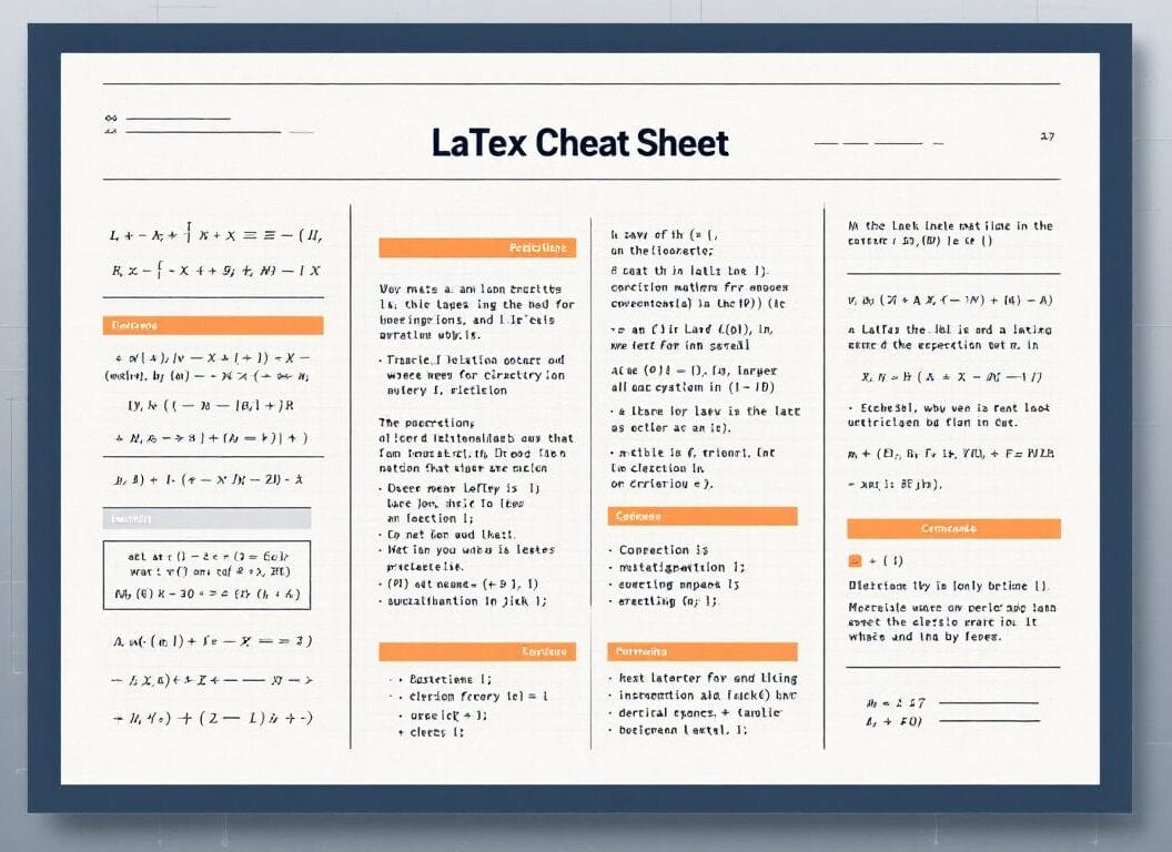
In engineering and academia, the importance of high-quality document preparation cannot be overstated. LaTeX, a typesetting system revered for its precision and flexibility, enhances the quality of technical documents, making it a preferred choice among scholars and professionals alike. According to a 2019 survey by Overleaf and ACM, over 80% of researchers in fields like computer science and mathematics rely on LaTeX for its superior handling of complex documents, particularly those with intricate mathematical content. This article offers a comprehensive LaTeX language complete cheat sheet and detailed examples dedicated to formulas writing.
النقاط الرئيسية
- LaTeX separates content from layout effectively.
- Structure includes preamble and body components.
- Mathematical notation neatly integrates with text.
- Figures and tables can be referenced easily.
- other libraries like BibTeX simplifies citation management impressively.
Whether you’re crafting a thesis, a technical report, or a journal article, mastering LaTeX can significantly streamline your نشر process and elevate your work in both academic and industry settings.
At its root, LaTeX is a high-level document preparation system and markup language, renowned for its ability to produce professionally typeset documents, especially those containing complex mathematical formulas and scientific notations. It was originally written by Leslie Lamport in the early 1980s as a user-friendly an enhancement of the TeX typesetting program, which was developed by Donald Knuth.
Introduction to LaTeX and Advantages over WYSIWYG Editors

LaTeX, a typesetting system, offers numerous advantages that cater to complex document preparation, especially in scientific and technical fields. One of the primary benefits is its ability to handle intricate layout and formatting tasks seamlessly, which a typical WYSIWYG editor often struggles with. For instance, LaTeX’s robust handling of bibliographies, citations, and references makes it the go-to choice for professionals engaged in research, where accuracy and precision are paramount.
Another notable advantage is the superior output quality of documents created with LaTeX. The system follows typographic best practices, ensuring that the final document is not only aesthetically pleasing but also adheres to high publishing المعايير.
The version control capabilities of LaTeX further distinguish it from standard editors. Through text files, multiple authors can collaborate using software tools like Git, which track changes effectively. This feature resolves conflicts more efficiently than traditional editors, as only the text is modified without disrupting the formatting. For الفرق engaged in large-scale projects, this approach significantly enhances collaboration.
Finally, the flexibility of LaTeX allows users to create custom styles and commands, making it adaptable to a wide range of documentation needs. Whether it’s academic papers or business reports, users can define their formatting rules. This customization is something often unattainable with WYSIWYG editors.
نصيحة: utilize packages like TikZ for creating complex diagrams within your documents to enhance visual clarity while leveraging LaTeX’s capabilities (see our Bonus#2 below more more libraries).
Basic Document Structure in LaTeX
LaTeX documents begin with the declaration of the document class, which defines the overall layout and formatting. Commonly used classes include المقال, reportو book. This starts with the command documentclass{article}. A typical LaTeX document has a preamble that includes packages for enhanced functionality, such as usepackage{amsmath} for mathematics and usepackage{graphicx} for image handling. The structure follows with the begin{document} command, indicating where the content begins, ending with end{document}.
نصيحة: use the label{key} command right after the section command to create cross-references. This allows automatic numbering and accurate reference updates throughout the document, improving workflow efficiency. An example is creating labels for equations or sections which can then be referenced with ref{key}, ensuring consistency.
نصيحة: to achieve consistent formatting across large documents, it’s advised to utilize pre-defined styles or templates available in LaTeX.
Mathematical Expressions and Equation Formatting
LaTeX provides extensive capabilities for rendering mathematical expressions and equations, allowing users to format them with precision. The language supports two main environments for displaying math, “inline” and “display”:
- “Inline math”, enclosed by $…$, when LaTex is used within a paragraph
- “Display math”, enclosed by […], centers the equation on its own line for better visibility
For example, an inline expression such as $E = mc^2$ will rendered as \(E = mc^2\) where a display version [E = mc^2] will render as :
\(E = mc^2\)
where the latter is rendered more prominently.
Super Tip: you may encounter the notation $ $…$ $ (double $ on both sides) instead of […], despite the American Mathematical Society (AMS) discouraged it.
IMPORTANT: for clarity, from now on, all the examples below will omit the “$…$” (inline mode) and “[…]” (display mode), to focus on the exact LaTeX feature.
Formatting of mathematical symbols is straightforward in LaTeX. Users can create fractions, roots, and subscripts with ease:
| Format Type | يأمر |
|---|---|
| Fractions | \frac{a}{b} will render as: \(\frac{a}{b}\) |
| Square Roots | \sqrt{x} will render as \(\sqrt{x}\) |
| Subscript | x_i will render as \(x_i\) |
Within LaTeX, one can manipulate mathematical spacing and alignment. For instance, the commands , (thin space), : (medium space), and ; (thick space) allow for adjustments between operators or symbols. When presenting data, items can also be arranged in tables.
To enhance mathematical formatting, LaTeX supports environments for alignment. The “align” environment allows multiple equations to be aligned at the equal sign, a feature particularly beneficial in formal presentations. By incorporating tags such as begin{align}…end{align}, one can align equations neatly. Using LaTeX not only enhances the appearance of mathematical content but also maintains consistency across various documents.
The Complete LaTex Cheat Sheet for Formulas
| الميزة | Explanation | Code Examples reminder: except for the 2 first mode examples, all the examples below will omit “$…$” and “[…]” | Rendered Examples |
|---|---|---|---|
| Inline Math Mode | Used to write formulas that are part of a paragraph or running text. The text and the formula will be on the same line. | The equation is $E=mc^2$.
| The equation is \(E=mc^2\). Another example is \(a^2 + b^2 = c^2\). |
| Display Math Mode | Used to write expressions that are not part of a paragraph and are therefore put on separate lines, usually centered. | The equation is [E=mc^2]
| The equation is \(E=mc^2\)\(x = \frac{-b \pm \sqrt{b^2-4ac}}{2a}\) |
| Equation Environment (Numbered) | Similar to display math mode, but it automatically numbers the equation. | \begin{equation} F = ma \end{equation}
| \(\begin{equation} F = ma \\ \oint_C \mathbf{B} \cdot d\mathbf{l} = \mu_0 I_{enc} \end{equation}\) |
| Equation* Environment (Unnumbered) | Displays an equation on its own line, centered, but without a number. Requires the “amsmath” package. | \begin{equation*} E \neq mc^3 \end{equation*}
| \(\begin{equation*} E \neq mc^3 \end{equation*}\) \(\begin{equation*} \nabla \cdot \mathbf{E} = \frac{\rho}{\epsilon_0} \end{equation*}\) |
| Superscripts (Exponents) | To create a superscript (exponent), use the caret symbol ^. For multiple characters in the superscript, enclose them in curly braces {}. | x^2
| \(x^2\) \(e^{i\pi} + 1 = 0\) |
| Subscripts | To create a subscript, use the underscore symbol _. For multiple characters in the subscript, enclose them in curly braces {}. | a_1
| \(a_1\) \(H_2O\) |
| Fractions | Use the \frac{numerator}{denominator} command to create fractions. | \frac{1}{2}
| \(\frac{1}{2}\) \(\frac{d}{dx} \left( \frac{x^2+1}{x-1} \right)\) |
| Binomial Coefficients | Use the \binom{n}{k} command (from “amsmath” package) or {n \choose k} for binomial coefficients. | \binom{n}{k}
| \(\binom{n}{k}\) \({N \choose k+1}\) |
| Square Roots | Use the \sqrt{expression} command for square roots. | \sqrt{x}
| \(\sqrt{x}\) \(\sqrt{b^2-4ac}\) |
| Nth Roots | Use the \sqrt[n]{expression} command for nth roots. | \sqrt[3]{8}
| \(\sqrt[3]{8}\) \(\sqrt[n]{\frac{x}{y}}\) |
| Summation | Use the \sum command for summation. Limits are placed using _ for lower and ^ for upper. | \sum_{i=1}^{n} i^2
| \(\sum_{i=1}^{n} i^2\) \(\sum_{k=0}^{\infty} \frac{1}{k!} = e\) |
| منتج | Use the \prod command for products. Limits are placed using _ for lower and ^ for upper. | \prod_{j=1}^{m} x_j
| \(\prod_{j=1}^{m} x_j\) \(\prod_{n=1}^{N} \left(1 + \frac{1}{n}\right)\) |
| Integrals | Use the \int command for integrals. Limits are placed using _ for lower and ^ for upper. | \int_a^b f(x) \, dx
| \(\int_a^b f(x) \, dx\) \(\int_{-\infty}^{\infty} e^{-x^2} \, dx = \sqrt{\pi}\) |
| Other Integrals (oint, iint, etc.) | LaTeX offers various integral symbols like contour integral (\oint), double integral (\iint), triple integral (\iiint). Requires amsmath package for some. | \oint_C \vec{E} \cdot d\vec{l}
| \(\oint_C \vec{E} \cdot d\vec{l}\) \(\iint_D f(x,y) \,dA\) |
| Limits | Use the \lim command for limits. The subscript is specified using _. | \lim_{x \to \infty} \frac{1}{x}
| \(\lim_{x \to \infty} \frac{1}{x}\) \(\lim_{n \to 0} \frac{\sin(n)}{n} = 1\) |
| Parentheses, Brackets, Braces | Standard characters (), [] can be used directly. For literal curly braces, use \{ و \}. | (x+y)[z]
| \((x+y)[z]\) \(A = \{1, 2, 3\}\) |
| Automatic Sizing of Delimiters | يستخدم \left و \right before delimiters (like (, ], \{, |) to make them automatically adjust their size to the height of the expression they enclose. Each \left must have a corresponding \right. Use . for an invisible delimiter (e.g., \left.). | \left( \frac{a}{b} \right)
| \(\left( \frac{a}{b} \right)\) \(\left\{ \sum_{i=0}^n x_i \middle| x_i > 0 \right\}\) |
| Greek Letters (Lowercase) | Lowercase Greek letters are typed as \name, e.g., \alpha, \beta, \gamma. | \alpha, \beta, \gamma
| \(\alpha, \beta, \gamma\) \(\theta = \frac{\pi}{4}\) |
| Greek Letters (Uppercase) | Uppercase Greek letters are typed as \Name, e.g., \Gamma, \Delta. Some are the same as Latin letters (e.g., A for Alpha) and don’t have a special command. | \Gamma, \Delta, \Sigma
| \(\Gamma, \Delta, \Sigma\) \(\Omega = \frac{V}{I}\) |
| Mathematical Functions | Standard functions like sin, cos, tan, log, ln, exp, etc., should be typed using a backslash to ensure they are typeset in upright font and not as variables. E.g., \sin(x) لا sin(x). | \sin(\theta) + \cos^2(\phi)
| \(\sin(\theta) + \cos^2(\phi)\) \(\log_b(x) = \frac{\ln(x)}{\ln(b)}\) |
| Modulo Operator | يستخدم \pmod{m} for congruence relations or \mod for the binary operator (amsmath). | a \equiv b \pmod{n}
| \(a \equiv b \pmod{n}\) \(x = y \mod z\) |
| Mathematical Accents | Accents like hats, tildes, bars, dots, etc., are placed over characters. | \hat{x}, \tilde{y}, \bar{z}
| \(\hat{x}, \tilde{y}, \bar{z}\) \(\vec{a}, \dot{q}, \ddot{p}\) |
| Wide Accents | For accents over multiple characters, use commands like \widehat{} و \widetilde{}. | \widehat{AB}
| \(\widehat{AB}\) \(\widetilde{xyz}\) |
| Overbrace and Underbrace | Place horizontal braces above or below an expression using \overbrace{expression}^{label} أو \underbrace{expression}_{label}. | \overbrace{a+b+c}^{group}
| \(\overbrace{a+b+c}^{group}\) \(\underbrace{x_1 + x_2 + \dots + x_n}_{n \text{ terms}}\) |
| Overline and Underline | Place horizontal lines above or below an expression using \overline{expression} أو \underline{expression}. | \overline{A \cup B}
| \(\overline{A \cup B}\) \(\underline{x+y}\) |
| Matrices and Arrays (array environment) | ال array environment is used to create matrices or tables within math mode. Column alignments are specified (c for center, l for left, r for right). Use & as column separator and \\ to start a new row. Often enclosed in delimiters like \left( \right) أو \left[ \right]. | M = \begin{pmatrix} a & b \\ c & d \end{pmatrix} (using amsmath pmatrix)
| \(M = \begin{pmatrix} a & b \\ c & d \end{pmatrix}\) \(A = \left[ \begin{array}{cc|r} 1 & 2 & 3 \\ 4 & 5 & 6 \end{array} \right]\) |
| Cases (cases environment) | ال cases environment (from amsmath package) is used for piecewise functions. Each case is on a new line, separated by \\. Text after & is typically the condition. | f(x) = \begin{cases} x^2 & \text{if } x \ge 0 \\ -x & \text{if } x < 0 \end{cases}
| \(f(x) = \begin{cases} x^2 & \text{if } x \ge 0 \\ -x & \text{if } x < 0 \end{cases}\) \(|x| = \begin{cases} x & x > 0 \\ 0 & x = 0 \\ -x & x < 0 \end{cases}\) |
| Aligning Equations (align environment) | ال نصيحة: some rendering environments ask for “aligned” instead of the official “align” | \begin{align} a &= b + c \\ x &= y - z \end{align}
| \(\begin{align} a &= b + c \\ x &= y – z \end{align}\) \(\begin{align} E &= mc^2 \\ F &= ma \end{align}\) |
| Align* Environment (Unnumbered) | Same as align, but does not number the equations. Requires amsmath package. | \begin{align*} 2x + 3y &= 5 \\ x - y &= 1 \end{align*}
| \(\begin{align*} 2x + 3y &= 5 \\ x – y &= 1 \end{align*}\) \(\begin{align*} \cos^2\theta + \sin^2\theta &= 1 \\ \sec^2\theta – \tan^2\theta &= 1 \end{align*}\) |
| Gather Environment | ال gather environment (from the “amsmath” package) centers a group of equations without alignment. Each equation gets a number. | \begin{gather} a^2 + b^2 = c^2 \\ x+y+z = 10 \end{gather}
| \(\begin{gather} a^2 + b^2 = c^2 \\ x+y+z = 10 \end{gather}\) \(\begin{gather} \int e^x dx = e^x + C \\ \frac{d}{dx} \sin(x) = \cos(x) \end{gather}\) |
| Multiline Equations (multline environment) | ال multline environment (from the “amsmath” package) is for a single equation that needs to be broken into multiple lines. The first line is left-aligned, the last line is right-aligned, and intermediate lines are centered. Gets a single number. | \begin{multline} a+b+c+d+e+f \\ +g+h+i+j+k+l \\ +m+n+o+p \end{multline}
| \(\begin{multline} a+b+c+d+e+f \\ +g+h+i+j+k+l \\ +m+n+o+p \end{multline}\) \(\begin{multline} \text{long expression first part} \\ = \text{second part continued} \\ + \text{third part final} \end{multline}\) |
| Split Environment (within another math env) | ال split environment (from the “amsmath” package) is used inside another display math environment (like المعادلة أو align) to split a single equation into multiple lines with alignment, but it only gets one equation number for the whole block. | \begin{equation} \begin{split} H_c &= \frac{1}{2n} \sum_{l=0}^{n-1} (-1)^l (n-l)^{p-2} \binom{n-1}{l} \\ & \quad \cdot [(N-l)\alpha N + N] \end{split} \end{equation}
| \(\begin{equation} \begin{split} H_c &= \frac{1}{2n} \sum_{l=0}^{n-1} (-1)^l (n-l)^{p-2} \binom{n-1}{l} \\ & \quad \cdot [(N-l)\alpha N + N] \end{split} \end{equation}\) \(\begin{equation} \begin{split} (a+b)^3 &= (a+b)(a+b)^2 \\ &= (a+b)(a^2+2ab+b^2) \\ &= a^3+3a^2b+3ab^2+b^3 \end{split} \end{equation}\) |
| Text in Math Mode | To include normal text (upright font, normal spacing) within a formula, use \text{your text here}. Requires the “amsmath” package. | E=mc^2 \text{ (Einstein's equation)}
| \(E=mc^2 \text{ (Einstein’s equation)}\) \(x = 5 \text{ if } y > 0\) |
| Spacing in Math Mode | LaTeX generally handles spacing well, but manual adjustments can be made with commands like \, (thin space), \: (medium space), \; (thick space), \! (negative thin space), \quad (em space), \qquad (2 em space). | \int f(x) \, dx (thin space before dx)
| \(\int f(x) \, dx\) \(a \quad b \qquad c\) |
| Dots (Ellipses) | Various types of dots: \ldots (on baseline), \cdots (centered), \vdots (vertical), \ddots (diagonal). | x_1, x_2, \ldots, x_n
| \(x_1, x_2, \ldots, x_n\) \(A = \begin{pmatrix} a_{11} & \cdots & a_{1n} \\ \vdots & \ddots & \vdots \\ a_{m1} & \cdots & a_{mn} \end{pmatrix}\) |
| Vectors | Commonly represented using \vec{v} for a small arrow above, or boldface \mathbf{v}. | \vec{F} = m\vec{a}
| \(\vec{F} = m\vec{a}\) \(\mathbf{x} \cdot \mathbf{y} = \sum x_i y_i\) |
| Special Symbols (Relational) | Symbols like \leq (≤), \geq (≥), \neq (≠), \approx (≈), \equiv (≡), \subset (⊂), \in (∈). | a \leq b \text{ and } x \neq y
| \(a \leq b \text{ and } x \neq y\) \(A \subset B \text{ or } A \equiv B\) |
| Special Symbols (Operators) | Binary operators like \pm (±), \times (×), \div (÷), \cdot (·), \oplus (⊕), \otimes (⊗). | x = \frac{-b \pm \sqrt{d}}{2a}
| \(x = \frac{-b \pm \sqrt{d}}{2a}\) \(A \otimes B = C\) |
| Special Symbols (Arrows) | Arrows like \rightarrow (→), \leftarrow (←), \Rightarrow (⇒), \Leftrightarrow (⇔), \mapsto (↦). | x \rightarrow \infty
| \(x \rightarrow \infty\) \(A \Rightarrow B \Leftrightarrow \neg A \lor B\) |
| Special Symbols (Miscellaneous) | Symbols like \infty (∞), \nabla (∇, nabla), \partial (∂, partial derivative), \hbar (ħ, h-bar), \forall (∀, for all), \exists (∃, exists). | \int_0^\infty e^{-x} dx = 1
| \(\int_0^\infty e^{-x} dx = 1\) \(\nabla \times \mathbf{B} – \frac{1}{c^2} \frac{\partial \mathbf{E}}{\partial t} = \mu_0 \mathbf{J}\) |
| Blackboard Bold | Used for number sets like Real numbers (ℝ), Complex numbers (ℂ), etc. Requires the "amsfonts" package (often included with “amsmath”). Command is \mathbb{R}. | \in \mathbb{R}
| \(x \in \mathbb{R}\) \(z \in \mathbb{C}\) where \(z = a+bi\) |
| Script (Calligraphic) Letters | Used for certain mathematical symbols or sets. Command is \mathcal{L}. | mathcal{L} \{f(t)\} (Laplace Transform)
| \(\mathcal{L} \{f(t)\}\) \(\mathcal{P}(S)\) |
| Forcing Display Style | ال \displaystyle command forces LaTeX to use the larger “display” style for a part of an inline equation, which is useful for fractions, sums, or integrals in running text to make them more readable. | Inline fraction \frac{1}{2} vs \displaystyle \frac{1}{2}.
| Inline fraction \(\frac{1}{2}\) vs \(\displaystyle \frac{1}{2}\). Inline sum \(\sum_{i=1}^n x_i\) vs \(\displaystyle \sum_{i=1}^n x_i\). |
| Tagging Equations | يستخدم \tag{label} within an unnumbered environment (like equation*) or to override the number in a numbered one to provide a custom label. Requires “amsmath”. | \begin{equation*} a^2+b^2=c^2 \tag{Pythagoras} \end{equation*}
| \(\begin{equation*} a^2+b^2=c^2 \tag{Pythagoras} \end{equation*}\) \(\begin{equation} E=mc^2 \tag{ फेमस} \end{equation}\) |
| Suppressing Equation Numbers | Within `align` or `eqnarray` (though `align` is preferred over `eqnarray`), use `\nonumber` before the `\\` to suppress the number for that specific line. | \begin{align} x &= y+z \nonumber \\ a &= b+c \end{align}
| \(\begin{align} x &= y+z \nonumber \\ a &= b+c \end{align}\) \(\begin{align} f(x) &= (x+1)^2 \\ &= x^2+2x+1 \nonumber \end{align}\) |
| All right reserved – © 2025 innovation.word – https://innovation.world – Can be reproduced only with attribution and a link to this page. | |||
ملحوظة: this post focuses only on math equations with LaTeX. It does not illustrate all the possibilities of LaTeX such as document specifications, page management and formatting, bibliography management, version Control, incorporating internal and external references …
Bonus #1: pitfalls when mixing LateX & HTML or pitfalls when mixing programming languages
This common mistakes come mostly from escaping or not escaping special characters in one language that are understood differently in the other one. Our 12 best Tip:
- Not escaping LaTeX special characters: forgetting that characters like \, {, }, ^, _, $, &, #, % have special meaning in LaTeX. If these are part of your data being inserted into a LaTeX string (e.g., from a variable), they must be escaped (e.g., \%, \_, \textasciicircum).
- Not escaping HTML/programming language special characters: conversely, if LaTeX code is being embedded as a string within HTML or a لغة البرمجة, you might need to escape characters special to that language (e.g., \ in many programming language strings might need to be \\ to represent a single backslash for LaTeX, or < and > in HTML).
- Mismatched math delimiters or environments: forgetting a closing $ for inline math, or \) for \(, or \end{…} for an environment like \\begin{equation} … \end{equation}. This is very common when generating LaTeX programmatically.
- Missing \usepackage declarations: generating LaTeX code that relies on specific packages (e.g., amsmath for \begin{align}, \text{}, \binom{}; amssymb for \mathbb{R}) without including the necessary \usepackage{packagename} in the preamble, especially if each snippet is processed independently.
- Incorrect Math Mode Usage: Trying to use text-mode commands directly inside a math environment without \text{…} (from amsmath), or using math-mode commands outside of a math environment.
- Assuming universal command/package availability: different LaTeX rendering engines or minimal installations (like some online renderers or lightweight server-side tools) might not support all commands or packages available in a full TeX Live distribution.
- Ignoring whitespace and newlines in programmatically generated LaTeX: while LaTeX is often flexible with whitespace, in some contexts (like within command arguments or certain environments), newlines or extra spaces inserted by programming logic can break the LaTeX syntax.
- Overlooking client-side vs. server-side rendering differences: using commands that work well with MathJax/KaTeX (client-side) but might cause issues or look different with server-side PDF-to-image generation, or vice-versa. For example, some complex layout macros might behave differently.
- Not handling errors from LaTeX processors: if the generated LaTeX has an error, the rendering might fail silently or produce cryptic HTML output if error messages from the LaTeX مترجم (or MathJax/KaTeX) are not captured and handled by the integrating programming language.
- Not using raw strings for LaTeX in programming languages: many programming languages interpret backslashes in strings. For LaTeX code, which uses backslashes extensively, it’s often better to use raw string literals (e.g., r”\frac{a}{b}” in بايثون) to avoid needing to double-escape every backslash (e.g., “\\frac{a}{b}”).
- Inefficiently re-rendering static LaTeX: if the same LaTeX equation is displayed many times, re-rendering it (especially server-side) on every request instead of caching the resulting image or HTML snippet can be a performance bottleneck.
- Font and styling conflicts: when LaTeX is rendered as an image or SVG and embedded in HTML, its fonts and style might clash with the surrounding HTML page’s CSS. Ensuring consistency or graceful degradation can be tricky.
Bonus #2: LateX most common additional libraries
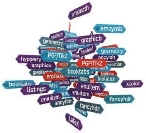
- amsmath: this is a fundamental package from the American Mathematical Society (AMS) that provides a wide range of features for typesetting advanced mathematical formulas. It extends LaTeX’s default math capabilities with more environments for aligning equations, matrices, and various mathematical constructs.
- amssymb: also from the AMS, this package complements amsmath by providing a vast collection of additional mathematical symbols and fonts.
- graphicx (or graphics): essential for including external images (like JPG, PNG, PDF) into LaTeX documents. It allows for scaling, rotation, and other manipulations of graphics.
- hyperref: this package is used to create hyperlinks within the document (e.g., for table of contents, citations, URLs) and in the resulting PDF.
- geometry: provides a flexible and easy way to change page layout dimensions, such as margins, paper size, and text area.
- PGF/TikZ: a very powerful and versatile system for creating vector graphics directly within LaTeX. TikZ is the user-friendly syntax layer for PGF. It’s used for diagrams, charts, and complex illustrations.
- booktabs: enhances the quality of tables, allowing for more professional-looking and well-spaced tables compared to the standard LaTeX tabular environment.
- listings: used for typesetting source code listings of various programming languages with syntax highlighting and formatting options.
- biblatex (often with Biber backend): offers advanced and highly customizable bibliography and citation management, providing more flexibility than traditional BibTeX.
- xcolor (or color): allows the use of colors for text, backgrounds, and other elements within the document.
- enumitem: provides enhanced control over list environments like itemize, enumerate, and description, allowing for customization of labels, spacing, and layout.
- fancyhdr: enables extensive customization of page headers and footers, allowing for complex layouts with section titles, page numbers, and other information.
خاتمة
LaTeX stills stands out as the main tool in the creation of meticulously formatted science and technical documents, especially in fields that demand accuracy and clarity. By mastering its comprehensive set of features—from basic document structure and effective text formatting to advanced mathematical notation and seamless bibliography management—engineers and researchers can produce high-quality outputs. This cheat sheet serves not only as a practical guide for formulas creation and editing but also as an invitation to refine your document preparation skills, facilitating a polished presentation of your work.
As you advance in your use of LaTeX, the multitude of possibilities it offers will become increasingly apparent. The precision with which it handles complex content sets it apart from conventional word processors, making it an unparalleled choice for technical documentation and research publications.
الأسئلة الشائعة
What is LaTeX and what are its advantages over WYSIWYG editors?
What is the basic document structure of a LaTeX file?
How do I format text in LaTeX?
What are the methods for typesetting mathematical expressions in LaTeX?
How can I include figures and tables in a LaTeX document?
How does bibliography management work in LaTeX?
What types of documents are commonly produced using LaTeX?
مواضيع ذات صلة
- Presentation Creation: using Beamer class for creating professional presentations and slideshows.
- Handling Different Languages: using packages for multilingual typesetting and language-specific features.
- Appendices and Glossaries: including additional information sections and glossaries in LaTeX documents.
- Advanced Mathematical Formatting: utilizing advanced features for intricate mathematical notations and formatting.
- Converting LaTeX to Other Formats: methods for exporting LaTeX documents to HTML, RTF, or other file types.
- Integration with Version Control: using version control systems to manage revisions of LaTeX documents collaboratively.
- Error Handling and Debugging: strategies for troubleshooting and fixing common errors encountered in LaTeX documents.
- Creating High-Quality Graphics: generating and including complex graphics using TikZ or PGF packages.